Tutorial - pastax

This tutorial walks through the core workflow of pastax on realistic, submesoscale-permitting, surface current fields read lazily from the IGE-MEOM OpenDAP:

Load a realistic surface ocean current (a Gulf-Stream subset of the eNATL60-BLBT02 simulation) and an overlying wind forcing, each kept on its own grid as a Dataset.
Deterministic trajectory simulation
1. Run a deterministic trajectory through the field with the solve ODE integrator, including a windage term.
2. Learn the windage coefficient thanks to JAX automatic differentiation, using optimistix to solve a least-square problem, and the separation distance as residual.
Stochastic trajectory ensemble simulation
1. Run a stochastic ensemble using a Smagorinsky diffusion on a smoothed copy of the current — exercising the SDE mode of solve and the Dataset.neighborhood API.
2. Jointly learn the windage and the Smagorinsky coefficient of a stochastic simulator, using a time-aggregated energy score with separation distance as kernel.
More “advanced” modelisation
1. Run a perturbed-ODE ensemble with a non-linear tanh-squashed noise residual — illustrating the ODE+controls pattern for implementing generative neural networks as simulators.
2. Run a second-order SDE with the full surface-ocean Maxey–Riley equation (a second-order PyTree (position, velocity) state, Coriolis, fluid acceleration and a wind/water-weighted carrier), perturbed by anisotropic eddy-diffusivity turbulence built as a lineax operator.

Boilerplate cells (imports, plot setup, animation rendering) are folded by default — click Show code to expand. The cells most relevant to the pastax API are always expanded.

import cartopy.crs as ccrs
import cmocean
import equinox as eqx
from IPython.display import HTML
import jax
jax.config.update("jax_enable_x64", True)
import jax.numpy as jnp
import jax.random as jr
from matplotlib import animation
import matplotlib.pyplot as plt
import numpy as np
import optimistix as optx
from scipy.ndimage import gaussian_filter
import xarray as xr

1. Loading the forcing fields¶

We load two forcing fields, each on its own grid:

the hourly ocean surface current $\mathbf{u}_o$ from a Gulf-Stream subset of the eNATL60-BLBT02 simulation (≈ 1/60°, 306 × 240 points, spanning 2010-02-11 → 2010-02-15), streamed from OpenDAP;
the 3-hourly 10 m wind $\mathbf{u}_w$ from the matching DFS5.2 forcing — a coarse 6 × 6 box covering the same region, also streamed from OpenDAP.

Because the two fields do not share a grid, they are kept as two Datasets and interpolated independently.

from pastax import degrees_to_meters

THREDDS = "https://ige-meom-opendap.univ-grenoble-alpes.fr/thredds"
OCEAN_URL = (f"{THREDDS}/dodsC/meomopendap/extract/MEOM/pastax-demo/"
             "eNATL60-BLBT02_y2010m02d11-2010m02d15.1h_SSUV_GS.nc")
WIND_URL = (f"{THREDDS}/dodsC/meomopendap/extract/MEOM/pastax-demo/"
            "wind_forcing_GS.nc")

o_ds = xr.open_dataset(OCEAN_URL)
w_ds = xr.open_dataset(WIND_URL)

NT, NY, NX = o_ds.sizes["time_counter"], o_ds.sizes["lat"], o_ds.sizes["lon"]

LAT = jnp.asarray(o_ds.lat.values)
LON = jnp.asarray(o_ds.lon.values)

DLAT = float(LAT[1] - LAT[0])
DLON = float(LON[1] - LON[0])
_m = degrees_to_meters(jnp.asarray([DLAT, DLON]), float(LAT.mean()))
DY_M, DX_M = float(_m[0]), float(_m[1])

LAT_W = jnp.asarray(w_ds.lat0.values)
LON_W = jnp.asarray(w_ds.lon0.values)

print("currents:", dict(o_ds.sizes), " wind:", dict(w_ds.sizes))
print(f"peak current speed: {float(np.sqrt(o_ds.u ** 2 + o_ds.v ** 2).max()):.2f} m/s")
print(f"peak wind speed:    {float(np.sqrt(w_ds.u10 ** 2 + w_ds.v10 ** 2).max()):.2f} m/s")

currents: {'time_counter': 120, 'lat': 224, 'lon': 233}  wind: {'time': 41, 'lat0': 6, 'lon0': 6}

peak current speed: 2.86 m/s
peak wind speed:    27.23 m/s

Animation of the joint forcing — the ocean current speed $\| \mathbf{u}_o \|$ is shown in colour; the wind $\mathbf{u}_w$ is overlaid as white arrows on its own coarse grid.

ocean_speed = (o_ds.u ** 2 + o_ds.v ** 2) ** 0.5
ocean_vmax = ocean_speed.quantile(0.98).values

PC = ccrs.PlateCarree()
EXTENT = [float(LON.min()), float(LON.max()), float(LAT.min()), float(LAT.max())]

fig, ax = plt.subplots(figsize=(7, 5), subplot_kw={"projection": PC})
plt.close(fig)

o_speed = ocean_speed.isel(time_counter=0)
time = o_speed.time_counter.values
im = ax.pcolormesh(LON, LAT, o_speed, cmap=cmocean.cm.ice,
                   vmin=0, vmax=ocean_vmax, shading="auto", transform=PC)
fig.colorbar(im, ax=ax, label=r"$\| \mathbf{u}_o \|$  (m s$^{-1}$)", extend="max")
q_w = ax.quiver(w_ds.lon0, w_ds.lat0,
                w_ds.u10.sel(time=time, method="nearest"), 
                w_ds.v10.sel(time=time, method="nearest"),
                scale=320, color="white", alpha=0.7, width=0.004, pivot="mid", transform=PC)
ax.set_extent(EXTENT, crs=PC)
title = ax.set_title(np.datetime_as_string(time, unit="s"))

def draw(k):
    global q_w
    o_speed = ocean_speed.isel(time_counter=k)
    time = o_speed.time_counter.values
    im.set_array(np.ravel(o_speed))
    q_w.remove()
    q_w = ax.quiver(w_ds.lon0, w_ds.lat0,
                    w_ds.u10.sel(time=time, method="nearest"), 
                    w_ds.v10.sel(time=time, method="nearest"),
                    scale=320, color="white", alpha=0.7, width=0.004, pivot="mid", transform=PC)
    title.set_text(np.datetime_as_string(time, unit="s"))
    return im, q_w, title

HTML(animation.FuncAnimation(fig, draw, frames=NT, interval=80, blit=False).to_jshtml())

Wrap each field into its own Dataset so the integrator can query them — forcing_ocean on the fine current grid and forcing_wind on the coarse wind grid. Dataset.from_xarray accepts forcings opened with xarray - note that those while be fully loaded in memory if opened lazily; for plain numpy or JAX arrays, use Dataset.from_arrays instead.

from pastax import Dataset

forcing_ocean = Dataset.from_xarray(
    o_ds,
    fields={"u_o": "u", "v_o": "v"},
    coordinates={"time": "time_counter", "lat": "lat", "lon": "lon"},
)
forcing_wind = Dataset.from_xarray(
    w_ds,
    fields={"u_w": "u10", "v_w": "v10"},
    coordinates={"time": "time", "lat": "lat0", "lon": "lon0"},
)

2. Deterministic trajectory simulation¶

1. A deterministic trajectory with windage¶

A surface object is advected by the ocean current and partially dragged by the wind. The direct windage model parameterises this as

\mathrm{d}\mathbf{X}(t) = \bigl[\mathbf{u}_o(t, \mathbf{X}) + \beta_w \, \mathbf{u}_w(t, \mathbf{X})\bigr] \, \mathrm{d}t,

(1)

with $\beta_w$ a dimensionless coefficient — typically 0.1 to $10\%$ depending on the object. Here we take $\beta_w = 3\%$ as ground truth.

In pastax the dynamics are expressed as a Python callable term(t, y, args) that returns the velocity in degrees per second. solve defaults to ODE mode and uses the Tsit5 integrator with a fixed step size.

from pastax import solve, Tsit5, meters_to_degrees

BETA_W_TRUE = 0.03  # 3% direct windage

def windage_term(t, y, args):
    # forcings and windage coefficient are passed through the `args` argument of `solve()`
    forcing_ocean, forcing_wind, beta_w = args
    lat_, lon_ = y[0], y[1]
    uo = forcing_ocean["u_o"].interp(t, lat_, lon_)
    vo = forcing_ocean["v_o"].interp(t, lat_, lon_)
    uw = forcing_wind["u_w"].interp(t, lat_, lon_)
    vw = forcing_wind["v_w"].interp(t, lat_, lon_)
    u = uo + beta_w * uw
    v = vo + beta_w * vw
    # convert (north=v, east=u) m/s -> (dlat/dt, dlon/dt) deg/s
    return meters_to_degrees(jnp.array([v, u]), lat_)

y0 = jnp.array([40.8, -61.2])                 # initial [lat, lon] -- western edge of the domain
ts_sim = forcing_ocean["u_o"].t_coords[1:-1]  # kept for plotting / indexing

# Derive solver parameters from ts_sim (avoids boundary timestamps)
t0_sim     = ts_sim[0]
n_save_sim = len(ts_sim) - 1
int_dt_sim = float(ts_sim[1] - ts_sim[0])

# CFL-limited integration sub-step: the real current is fast (~2-3 m/s) on a ~1.5 km
# grid, so we integrate with several sub-steps per saved hour (save_dt stays int_dt_sim).
CFL = 0.5
u_max = float(jnp.sqrt(
    forcing_ocean["u_o"].values ** 2 + forcing_ocean["v_o"].values ** 2
).max())
n_sub = int(np.ceil(int_dt_sim / (CFL * min(DX_M, DY_M) / u_max)))
INT_DT = int_dt_sim / n_sub

traj = solve(windage_term, y0,
             t0_sim, n_save_sim, INT_DT, int_dt_sim, solver=Tsit5(),
             args=(forcing_ocean, forcing_wind, BETA_W_TRUE))
print("trajectory shape:", traj.shape, " sub-steps/hour:", n_sub)

trajectory shape: (118, 2)  sub-steps/hour: 15

Animation — the time-evolving ocean speed and wind velocity underneath, the trajectory growing one step at a time.

fig, ax = plt.subplots(figsize=(7, 5), subplot_kw={"projection": PC})
plt.close(fig)

o_speed = ocean_speed.isel(time_counter=0)
time = o_speed.time_counter.values
im = ax.pcolormesh(LON, LAT, o_speed, cmap=cmocean.cm.ice,
                   vmin=0, vmax=ocean_vmax, shading="auto", transform=PC)
fig.colorbar(im, ax=ax, label=r"$\| \mathbf{u}_o \|$  (m s$^{-1}$)", extend="max")
q_w = ax.quiver(w_ds.lon0, w_ds.lat0,
                w_ds.u10.sel(time=time, method="nearest"), 
                w_ds.v10.sel(time=time, method="nearest"),
                scale=320, color="white", alpha=0.7, width=0.004, pivot="mid", transform=PC)
line, = ax.plot([], [], color="gold", lw=2, transform=PC)
ax.scatter([y0[1]], [y0[0]], color="gold", zorder=4, s=20, transform=PC)
ax.set_extent(EXTENT, crs=PC)
title = ax.set_title(np.datetime_as_string(time, unit="s"))

# match field timestep to trajectory timestep (ts_sim starts at index 1)
def draw(k):
    global q_w
    field_k = k + 1
    o_speed = ocean_speed.isel(time_counter=field_k)
    time = o_speed.time_counter.values
    im.set_array(np.ravel(o_speed))
    q_w.remove()
    q_w = ax.quiver(w_ds.lon0, w_ds.lat0,
                    w_ds.u10.sel(time=time, method="nearest"), 
                    w_ds.v10.sel(time=time, method="nearest"),
                    scale=320, color="white", alpha=0.7, width=0.004, pivot="mid", transform=PC)
    line.set_data(traj[: k + 1, 1], traj[: k + 1, 0])
    title.set_text(np.datetime_as_string(time, unit="s"))
    return im, line, q_w, title

HTML(animation.FuncAnimation(fig, draw, frames=len(traj), interval=80, blit=False).to_jshtml())

2. Learning the windage coefficient¶

pastax’s solve is fully differentiable. We exploit that to fit the parameters of a term function: given a reference trajectory $\mathbf{Y}^*$ produced by the true dynamics, recover the parameters of a model that matches it.

We start with the deterministic case: recover the windage coefficient $\beta_w$ from a single trajectory, using the per-time separation distance between simulated and reference paths as residuals. The model uses the (perfectly observed) true ocean and wind fields but a tunable $\beta_w$ ; the reference trajectory is generated with $\beta_w = 3\%$ .

class TunableWindage(eqx.Module):
    beta_w: jax.Array

    def __call__(self, t, y, args):
        forcing_ocean, forcing_wind = args
        return windage_term(t, y, (forcing_ocean, forcing_wind, self.beta_w))

    def get_physical_beta_w(self):
        return self.beta_w

term_init = TunableWindage(beta_w=jnp.array(0.0))

# Reference trajectory: true windage on the true ocean+wind forcing
true_traj = solve(windage_term, y0,
                  t0_sim, n_save_sim, INT_DT, int_dt_sim, solver=Tsit5(),
                  args=(forcing_ocean, forcing_wind, BETA_W_TRUE))

# Initial estimate: tunable term with beta_w = 1.5%
init_traj = solve(term_init, y0,
                  t0_sim, n_save_sim, INT_DT, int_dt_sim, solver=Tsit5(),
                  args=(forcing_ocean, forcing_wind))
print("ref shape:", true_traj.shape, "  init shape:", init_traj.shape)

ref shape: (118, 2)   init shape: (118, 2)

from pastax import Heun, separation_distance

@eqx.filter_jit
def residual_fn(term_module, ref_traj):
    # Levenberg-Marquardt builds the residual Jacobian in forward mode (jvp), so we
    # opt into adjoint="forward" — the default "checkpointed" adjoint is reverse-mode only.
    est_traj = solve(term_module, y0,
                     t0_sim, n_save_sim, INT_DT, int_dt_sim, solver=Heun(),
                     args=(forcing_ocean, forcing_wind), adjoint="forward")
    return separation_distance(est_traj, ref_traj)  # (T,) residuals in metres

solver = optx.BestSoFarLeastSquares(optx.LevenbergMarquardt(rtol=1e-4, atol=1e-4))
sol = optx.least_squares(residual_fn, solver=solver, y0=term_init, args=true_traj)
term_fit = sol.value
print(f"stopped after {int(sol.stats['num_steps'])} steps  ->  "
      f"beta_w = {float(term_fit.get_physical_beta_w()) * 100:.1f}%")
print(f"truth                   ->  beta_w = {BETA_W_TRUE * 100:.1f}%")

stopped after 64 steps  ->  beta_w = 3.0%
truth                   ->  beta_w = 3.0%

Animation — the truth, the initial guess, and the fitted trajectory drawn together over the time-evolving ocean speed and wind velocity.

final_traj = solve(term_fit, y0,
                   t0_sim, n_save_sim, INT_DT, int_dt_sim, solver=Tsit5(),
                   args=(forcing_ocean, forcing_wind))

fig, ax = plt.subplots(figsize=(7, 5), subplot_kw={"projection": PC})
plt.close(fig)

o_speed = ocean_speed.isel(time_counter=0)
time = o_speed.time_counter.values
im = ax.pcolormesh(LON, LAT, o_speed, cmap=cmocean.cm.ice,
                   vmin=0, vmax=ocean_vmax, shading="auto", transform=PC)
fig.colorbar(im, ax=ax, label=r"$\| \mathbf{u}_o \|$  (m s$^{-1}$)", extend="max")
q_w = ax.quiver(w_ds.lon0, w_ds.lat0,
                w_ds.u10.sel(time=time, method="nearest"), 
                w_ds.v10.sel(time=time, method="nearest"),
                scale=320, color="white", alpha=0.7, width=0.004, pivot="mid", transform=PC)

l_true,  = ax.plot([], [], color="gold", lw=2.0, label="Truth", transform=PC)
l_init,  = ax.plot([], [], color="orange", lw=1.5, ls="--", 
                   label=r"Initial ($\beta_w = $" + f"{float(term_init.get_physical_beta_w()) * 100:.1f}%" + r"$)$", 
                   transform=PC)
l_final, = ax.plot([], [], color="red", lw=2.0, ls=":",  label="Fitted", transform=PC)
ax.scatter([y0[1]], [y0[0]], color="gold", zorder=4, s=20, transform=PC)
ax.set_extent(EXTENT, crs=PC)
ax.legend(loc="upper right", fontsize=8)
title = ax.set_title(np.datetime_as_string(time, unit="s"))

def draw(k):
    global q_w
    field_k = k + 1
    o_speed = ocean_speed.isel(time_counter=field_k)
    time = o_speed.time_counter.values
    im.set_array(np.ravel(o_speed))
    q_w.remove()
    q_w = ax.quiver(w_ds.lon0, w_ds.lat0,
                    w_ds.u10.sel(time=time, method="nearest"), 
                    w_ds.v10.sel(time=time, method="nearest"),
                    scale=320, color="white", alpha=0.7, width=0.004, pivot="mid", transform=PC)
    l_true.set_data(true_traj[: k + 1, 1], true_traj[: k + 1, 0])
    l_init.set_data(init_traj[: k + 1, 1], init_traj[: k + 1, 0])
    l_final.set_data(final_traj[: k + 1, 1], final_traj[: k + 1, 0])
    title.set_text(np.datetime_as_string(time, unit="s"))
    return im, q_w, l_true, l_init, l_final, title

HTML(animation.FuncAnimation(fig, draw, frames=len(true_traj), interval=80, blit=False).to_jshtml())

3. Stochastic trajectory ensemble simulation¶

1. A stochastic ensemble with Smagorinsky diffusion¶

In a real setting the gridded ocean current we feed the simulator is smoothed relative to the actual flow a drifter feels -- think of altimetry-derived surface currents, which only resolve the mesoscale. From here on the model therefore runs on $\widetilde{\mathbf{u}}_o$ , a smoothed copy of $\mathbf{u}_o$ , and the role of a stochastic term is to compensate for the small-scale features the gridded field misses.

# Smooth the eNATL60 current to a GLORYS-like (~1/12°) effective resolution: a Gaussian
# low-pass removes the submesoscale that the stochastic model will instead represent as
# diffusion, then we resample onto a coarser 1/12-degree grid.
SMOOTH_SIGMA = 3.5  # gaussian sigma, in fine-grid cells
u_o_lp = gaussian_filter(o_ds.u.values, 
                         sigma=(0.5, SMOOTH_SIGMA, SMOOTH_SIGMA), mode="nearest")
v_o_lp = gaussian_filter(o_ds.v.values, 
                         sigma=(0.5, SMOOTH_SIGMA, SMOOTH_SIGMA), mode="nearest")

RES_S = 1.0 / 12.0  # target resolution (deg)
LAT_S = jnp.arange(float(LAT.min()), float(LAT.max()) + 1e-9, RES_S)
LON_S = jnp.arange(float(LON.min()), float(LON.max()) + 1e-9, RES_S)
o_smooth_ds = xr.Dataset(
    {"u": (("t", "lat", "lon"), u_o_lp), "v": (("t", "lat", "lon"), v_o_lp)},
    coords={"t": o_ds.time_counter.values, "lat": LAT, "lon": LON},
).interp(lat=np.asarray(LAT_S), lon=np.asarray(LON_S))

DLAT_S = float(LAT_S[1] - LAT_S[0])
DLON_S = float(LON_S[1] - LON_S[0])
_ms = degrees_to_meters(jnp.asarray([DLAT_S, DLON_S]), float(LAT_S.mean()))
DY_M_S, DX_M_S = float(_ms[0]), float(_ms[1])

forcing_ocean_smooth = Dataset.from_xarray(
    o_smooth_ds,
    fields={"u_o": "u", "v_o": "v"},
    coordinates={"time": "t", "lat": "lat", "lon": "lon"},
)
ocean_speed_smooth = (o_smooth_ds.u ** 2 + o_smooth_ds.v ** 2) ** 0.5

# Deterministic windage on the smoothed currents: the drift the ensemble spreads around.
traj_smooth = solve(windage_term, y0,
                    t0_sim, n_save_sim, INT_DT, int_dt_sim, solver=Tsit5(),
                    args=(forcing_ocean_smooth, forcing_wind, BETA_W_TRUE))

print("smoothing reduced peak ocean speed from "
      f"{float(np.sqrt(o_ds.u ** 2 + o_ds.v ** 2).max()):.2f} to "
      f"{float(np.sqrt(o_smooth_ds.u ** 2 + o_smooth_ds.v ** 2).max()):.2f} m/s "
      f"(grid {NY}x{NX} -> {LAT_S.size}x{LON_S.size})")

smoothing reduced peak ocean speed from 2.86 to 2.28 m/s (grid 224x233 -> 45x47)

Sub-grid turbulence the smoothed $\mathbf{u}_o$ does not resolve is conventionally reintroduced as a stochastic diffusion with a Smagorinsky-style local turbulent viscosity:

K(\mathbf{x}, t) = C_S \, \Delta x^2 \sqrt{2(\partial_x u)^2 + 2(\partial_y v)^2 + (\partial_y u + \partial_x v)^2},

(2)

estimated from a $3 \times 3$ patch of the smoothed current via Dataset.neighborhood. With the solver’s Wiener-increment convention $\mathrm{d}\mathbf{W} = \sqrt{\Delta t}\,\mathbf{z}$ and $\mathbf{z} \sim \mathcal{N}(0, I_2)$ , the diffusion coefficient that produces a per-step displacement variance of $2K\,\Delta t$ is $\sigma = \sqrt{2K}$ — the $\Delta t$ factor lives in the increment, not in the coefficient.

We switch to SDE mode by passing key to solve. In SDE mode the term has the signature term(t, y, args) -> (drift, g): it returns the deterministic velocity and the diffusion coefficient $g(t, y)$ separately. The solver draws $\mathbf{z} \sim \mathcal{N}(0, I_2)$ and applies $\mathbf{g}\,\mathrm{d}\mathbf{W}$ internally — the term never receives $\mathbf{z}$ . An ensemble of 100 independent realisations is obtained by passing n_samples=100; solve splits the key internally. We use the Stratonovich Heun solver — its predictor–corrector reuses the same Wiener increment across both stages.

from pastax import Heun, safe_sqrt

CS = 0.1  # Smagorinsky coefficient

def smag_windage_term(t, y, args):
    forcing_ocean, forcing_wind, beta_w, c_s = args
    lat_, lon_ = y[0], y[1]

    uo = forcing_ocean["u_o"].interp(t, lat_, lon_)
    vo = forcing_ocean["v_o"].interp(t, lat_, lon_)
    uw = forcing_wind["u_w"].interp(t, lat_, lon_)
    vw = forcing_wind["v_w"].interp(t, lat_, lon_)
    u = uo + beta_w * uw
    v = vo + beta_w * vw
    drift = meters_to_degrees(jnp.array([v, u]), lat_)

    # 3x3 patch of the smoothed current (1/12-degree grid -> use its spacing DX_M_S/DY_M_S).
    patches = forcing_ocean.neighborhood(t, lat_, lon_, t_window=0, lat_window=1, lon_window=1)
    u_p = patches["u_o"][0]
    v_p = patches["v_o"][0]
    du_dx = (u_p[1, 2] - u_p[1, 0]) / (2 * DX_M_S)
    du_dy = (u_p[2, 1] - u_p[0, 1]) / (2 * DY_M_S)
    dv_dx = (v_p[1, 2] - v_p[1, 0]) / (2 * DX_M_S)
    dv_dy = (v_p[2, 1] - v_p[0, 1]) / (2 * DY_M_S)

    strain = safe_sqrt(2 * du_dx ** 2 + 2 * dv_dy ** 2 + (du_dy + dv_dx) ** 2)
    K = c_s * DX_M_S ** 2 * strain
    sigma = safe_sqrt(2 * K)
    g = meters_to_degrees(jnp.array([sigma, sigma]), lat_)

    return drift, g

# n_samples=100 splits the key internally and returns shape (100, n_save+1, 2).
ensemble = solve(smag_windage_term, y0,
                 t0_sim, n_save_sim, INT_DT, int_dt_sim, solver=Heun(),
                 args=(forcing_ocean_smooth, forcing_wind, BETA_W_TRUE, CS),
                 key=jr.key(0), n_samples=100)
print("ensemble shape:", ensemble.shape)

/opt/hostedtoolcache/Python/3.11.15/x64/lib/python3.11/site-packages/jax/_src/ops/scatter.py:105: FutureWarning: scatter inputs have incompatible types: cannot safely cast value from dtype=float64 to dtype=float32 with jax_numpy_dtype_promotion=standard. In future JAX releases this will result in an error.
  warnings.warn(

ensemble shape: (100, 118, 2)

Animation — each thin red line is one stochastic realisation; the dashed red line is the deterministic, diffusion-free windage trajectory on the same smoothed currents. Both are drawn over the time-evolving smoothed ocean speed and wind velocity.

fig, ax = plt.subplots(figsize=(7, 5), subplot_kw={"projection": PC})
plt.close(fig)

o_speed = ocean_speed_smooth.isel(t=0)
time = o_speed.t.values
im = ax.pcolormesh(LON_S, LAT_S, o_speed, cmap=cmocean.cm.ice,
                   vmin=0, vmax=ocean_vmax, shading="auto", transform=PC)
fig.colorbar(im, ax=ax, label=r"$\| \widetilde{\mathbf{u}}_o \|$  (m s$^{-1}$)", extend="max")
q_w = ax.quiver(w_ds.lon0, w_ds.lat0,
                w_ds.u10.sel(time=time, method="nearest"), 
                w_ds.v10.sel(time=time, method="nearest"),
                scale=320, color="white", alpha=0.7, width=0.004, pivot="mid", transform=PC)

ens_lines = [ax.plot([], [], color="red", alpha=0.18, lw=0.6, transform=PC)[0]
             for _ in range(ensemble.shape[0])]
l_true, = ax.plot([], [], color="gold", lw=2.0, label="Truth", transform=PC)
det_line, = ax.plot([], [], color="red", lw=1.5, ls="--", label="Deterministic", transform=PC)
ax.plot([], [], color="red", lw=0.6, label="Stochastic", transform=PC)
ax.scatter([y0[1]], [y0[0]], color="gold", zorder=4, s=20, transform=PC)
ax.set_extent(EXTENT, crs=PC)
ax.legend(loc="upper right", fontsize=8)
title = ax.set_title(np.datetime_as_string(time, unit="s"))

def draw(k):
    global q_w
    field_k = k + 1
    o_speed = ocean_speed_smooth.isel(t=field_k)
    time = o_speed.t.values
    im.set_array(np.ravel(o_speed))
    q_w.remove()
    q_w = ax.quiver(w_ds.lon0, w_ds.lat0,
                    w_ds.u10.sel(time=time, method="nearest"), 
                    w_ds.v10.sel(time=time, method="nearest"),
                    scale=320, color="white", alpha=0.7, width=0.004, pivot="mid", transform=PC)
    for i, ln in enumerate(ens_lines):
        ln.set_data(ensemble[i, : k + 1, 1], ensemble[i, : k + 1, 0])
    l_true.set_data(true_traj[: k + 1, 1], true_traj[: k + 1, 0])
    det_line.set_data(traj_smooth[: k + 1, 1], traj_smooth[: k + 1, 0])
    title.set_text(np.datetime_as_string(time, unit="s"))
    return [im, q_w, l_true, det_line, title, *ens_lines]

HTML(animation.FuncAnimation(fig, draw, frames=ensemble.shape[1], interval=80, blit=False).to_jshtml())

2. Jointly learning windage and diffusion¶

In the previous section we set the Smagorinsky constant $C_S$ to an arbitrary value of 0.1. Here we will recover $(\beta_w, C_S)$ jointly.

We set this up by:

using the smoothed currents of §3.1 (forcing_smooth) as the observed forcing;
generating 10 deterministic reference trajectories with leeway $\beta_w^* = 3\%$ on the unsmoothed currents, seeded in the left side of the domain. Each one is treated as a single sample from the true distribution (the distribution induced by the unresolved scales we are about to parameterise away);
fitting the model -- which uses the smoothed currents plus a Smagorinsky SDE -- by minimising the time-aggregated energy score–see Pic, R., Dombry, C., Naveau, P., and Taillardat, M. (2025, Adv. Stat. Clim. Meteorol. Oceanogr.)–with separation distance as kernel, summed over all 10 reference trajectories:

\mathrm{ES}_t(F, y^*_t) = \frac{1}{M} \sum_{i=1}^M d(X^{(i)}_t, y^*_t) \;-\; \frac{1}{2M(M-1)} \sum_{i \neq j} d(X^{(i)}_t, X^{(j)}_t), \qquad \mathcal{L} = \sum_{k=1}^{K=10} \sum_t \mathrm{ES}_t(F_n, y^{*,k}_t).

(3)

We do not have a ground-truth $C_S$ -- $C_S$ is a parameterisation knob, not a physical constant of the unsmoothed flow. We start from a non-zero value and ask the optimiser to move it without collapsing it to zero.

The energy score, alongside the squared error, Dawid-Sebastiani score, and variogram score, ships in pastax.score as a proper scoring rule for ensemble forecasts. Each accepts a reduce={None, "last", "sum"} argument and per-time weights; squared_error and energy_score additionally accept any broadcasting distance kernel -- here we plug in pastax.separation_distance for great-circle distances on the sphere.

# --- 10 reference trajectories seeded randomly in the western part of the domain ---
N_REFERENCES = 10
key = jr.key(0)
subkey, key = jr.split(key)
y0s_ref = jax.random.uniform(subkey, (N_REFERENCES, 2),
                             minval=jnp.array([LAT.min() + 1.5, LON.min() + 0.05]),
                             maxval=jnp.array([LAT.max() - 0.5, LON.min() + 1.5]))

# Reference trajectories: deterministic windage on the *true* (unsmoothed) currents.
ref_trajs = jax.vmap(
    lambda y0_i: solve(windage_term, y0_i,
                       t0_sim, n_save_sim, INT_DT, int_dt_sim, solver=Heun(),
                       args=(forcing_ocean, forcing_wind, BETA_W_TRUE))
)(y0s_ref)

# If a trajectory leaves the domain, we resample a new initial point and recompute it
is_out_of_bounds = lambda traj: jnp.any((jnp.logical_or(traj[:, 0] < LAT.min(), traj[:, 0] > LAT.max())) |
                                        (jnp.logical_or(traj[:, 1] < LON.min(), traj[:, 1] > LON.max())))
out_of_bounds_mask = jax.vmap(is_out_of_bounds)(ref_trajs)
while jnp.any(out_of_bounds_mask):
    n_out = int(out_of_bounds_mask.sum())
    subkey, key = jr.split(key)
    new_y0s = jax.random.uniform(subkey, (n_out, 2),
                                 minval=jnp.array([LAT.min() + 1.5, LON.min() + 0.05]),
                                 maxval=jnp.array([LAT.max() - 0.5, LON.min() + 1.5]))
    y0s_ref = y0s_ref.at[out_of_bounds_mask].set(new_y0s)
    ref_trajs = jax.vmap(
        lambda y0_i: solve(windage_term, y0_i,
                           t0_sim, n_save_sim, INT_DT, int_dt_sim, solver=Heun(),
                           args=(forcing_ocean, forcing_wind, BETA_W_TRUE))
    )(y0s_ref)
    out_of_bounds_mask = jax.vmap(is_out_of_bounds)(ref_trajs)

print("ref_trajs shape:", ref_trajs.shape)

# --- Tunable model: smoothed currents + Smagorinsky SDE ---
class TunableStoch(eqx.Module):
    beta_w_pct: jax.Array  # beta_w stored in percent (O(1))
    c_s_x10:    jax.Array  # c_s   stored *10        (O(1))

    @property
    def beta_w(self):
        return self.beta_w_pct * 0.01
    @property
    def c_s(self):
        return self.c_s_x10 * 0.1

    def __call__(self, t, y, args):
        forcing_ocean, forcing_wind = args
        return smag_windage_term(t, y, (forcing_ocean, forcing_wind, self.beta_w, self.c_s))

# Initial guess: a non-zero C_S. We have no ground truth for it; the optimiser
# should move it without collapsing it to zero.
stoch_init = TunableStoch(beta_w_pct=jnp.array(0.0), c_s_x10=jnp.array(1.0))

ref_trajs shape: (10, 118, 2)

from pastax import energy_score

# `energy_score(ens, ref, kernel=separation_distance, reduce="sum")` returns the
# time-aggregated energy score with great-circle distance as kernel:
#   ES = sum_t [ mean_m d(X^m, y_t)  -  sum_{i!=j} d(X^i, X^j) / (2 M (M-1)) ]

M = 10  # ensemble members per trajectory

@eqx.filter_jit
def stoch_loss(term_module, args):
    refs, key = args
    keys = jr.split(key, N_REFERENCES)
    def per(y0_i, k_i, r_i):
        ens = solve(term_module, y0_i,
                    t0_sim, n_save_sim, INT_DT, int_dt_sim, solver=Heun(),
                    args=(forcing_ocean_smooth, forcing_wind),
                    key=k_i, n_samples=M)
        return energy_score(ens, r_i, kernel=separation_distance, reduce="sum")
    return jnp.sum(jax.vmap(per)(y0s_ref, keys, refs))

solver_joint = optx.BestSoFarMinimiser(optx.BFGS(rtol=1e-4, atol=1e-4))
sol_joint = optx.minimise(
    stoch_loss, solver=solver_joint, y0=stoch_init,
    args=(ref_trajs, jr.key(0)), throw=False,
)
beta_fit_joint = float(sol_joint.value.beta_w)
cs_fit_joint   = float(sol_joint.value.c_s)
print(f"stopped after {int(sol_joint.stats['num_steps'])} steps  -> "
      f"beta_w = {beta_fit_joint * 100:.1f}%, "
      f"C_S = {cs_fit_joint:.3f}")
print(f"truth                   -> beta_w = {BETA_W_TRUE * 100:.1f}% (no true C_S)")

stoch_fit = sol_joint.value

stopped after 68 steps  -> beta_w = 3.0%, C_S = 0.067
truth                   -> beta_w = 3.0% (no true C_S)

Animation -- the 10 deterministic reference trajectories drawn against the smoothed ocean current the model actually sees, each surrounded by a 30-member SDE ensemble drawn from the fitted parameters.

ENS_SHOW = 30  # ensemble members per reference to draw

ens_show = jax.vmap(
    lambda y0_i, k_i: solve(stoch_fit, y0_i,
                             t0_sim, n_save_sim, INT_DT, int_dt_sim, solver=Heun(),
                             args=(forcing_ocean_smooth, forcing_wind),
                             key=k_i, n_samples=ENS_SHOW)
)(y0s_ref, jr.split(jr.key(7), N_REFERENCES))

fig, ax = plt.subplots(figsize=(7, 5), subplot_kw={"projection": PC})
plt.close(fig)

o_speed = ocean_speed_smooth.isel(t=0)
time = o_speed.t.values
im = ax.pcolormesh(LON_S, LAT_S, o_speed, cmap=cmocean.cm.ice,
                   vmin=0, vmax=ocean_vmax, shading="auto", transform=PC)
fig.colorbar(im, ax=ax, label=r"$\| \widetilde{\mathbf{u}}_o \|$  (m s$^{-1}$)", extend="max")
q_w = ax.quiver(w_ds.lon0, w_ds.lat0,
                w_ds.u10.sel(time=time, method="nearest"), 
                w_ds.v10.sel(time=time, method="nearest"),
                scale=320, color="white", alpha=0.7, width=0.004, pivot="mid", transform=PC)

colors = plt.cm.spring(np.linspace(0, 1, N_REFERENCES))
ens_lines = [[ax.plot([], [], color=colors[d], alpha=0.5, lw=0.5, transform=PC)[0]
              for _ in range(ENS_SHOW)]
             for d in range(N_REFERENCES)]
ref_lines = [ax.plot([], [], color=colors[d], lw=2.0, transform=PC)[0]
             for d in range(N_REFERENCES)]
ax.plot([], [], color="k", lw=2.0, label="Truth", transform=PC)
ax.plot([], [], color="k", lw=0.5, alpha=0.75, label="Simulated", transform=PC)
_ = [ax.scatter(ref_trajs[d, 0, 1], ref_trajs[d, 0, 0], color=colors[d], zorder=4, s=20, transform=PC)
      for d in range(N_REFERENCES)]
ax.set_extent(EXTENT, crs=PC)
ax.legend(loc="upper right", fontsize=8)
title = ax.set_title(np.datetime_as_string(time, unit="s"))

def draw(k):
    global q_w
    field_k = k + 1
    o_speed = ocean_speed_smooth.isel(t=field_k)
    time = o_speed.t.values
    im.set_array(np.ravel(o_speed))
    q_w.remove()
    q_w = ax.quiver(w_ds.lon0, w_ds.lat0,
                    w_ds.u10.sel(time=time, method="nearest"), 
                    w_ds.v10.sel(time=time, method="nearest"),
                    scale=320, color="white", alpha=0.7, width=0.004, pivot="mid", transform=PC)
    for d in range(N_REFERENCES):
        ref_lines[d].set_data(ref_trajs[d, : k + 1, 1], ref_trajs[d, : k + 1, 0])
        for j, ln in enumerate(ens_lines[d]):
            ln.set_data(ens_show[d, j, : k + 1, 1],
                        ens_show[d, j, : k + 1, 0])
    title.set_text(np.datetime_as_string(time, unit="s"))
    return [im, q_w, title, *ref_lines, *[ln for grp in ens_lines for ln in grp]]

HTML(animation.FuncAnimation(fig, draw, frames=ens_show.shape[2],
                             interval=80, blit=False).to_jshtml())

4. More “advanced” modelisation¶

1. A stochastic ensemble via perturbed ODE¶

The SDE approach above hard-wires a linear noise model: the per-step displacement is $\mathbf{g}(t, \mathbf{X})\,\mathrm{d}\mathbf{W}$ , a linear function of the Wiener increment. More expressive stochastic samplers — such as generative neural networks — learn a non-linear mapping $\mathbf{z} \mapsto \boldsymbol{\varepsilon}$ from a standard-normal seed to a richer, possibly multi-modal displacement distribution. The SDE solver cannot represent this: it always computes $\mathbf{g} \cdot \mathrm{d}\mathbf{W}$ .

The ODE+controls pattern handles it directly. The user pre-samples a batch of noise trajectories (shape (S, n_fine, 2)) from any distribution and vmaps solve over them; each integration step receives one ctrl slice and the term applies whatever non-linear transform it likes. The solver never sees the noise — it simply multiplies the returned velocity by $\Delta t$ .

Here we illustrate with a tanh-squashed Gaussian: ctrl ~ N(0, I_2) is mapped through $\tanh$ before being scaled by the local Smagorinsky amplitude $g$ . Compared to the linear SDE this produces a bounded residual velocity (no arbitrarily large steps), while retaining the correct local scale. Replacing tanh with a generative neural network requires no changes to the solver or the integration loop.

def perturbed_ode_term(t, y, args, ctrl):
    drift, g = smag_windage_term(t, y, args)
    z = ctrl
    # Non-linear transform: tanh squashes z ~ N(0, I_2) into (-1, 1),
    # giving a bounded residual. Swap tanh for an neural network to get a
    # richer distribution — the solver and integration loop are unchanged.
    residual = g * jnp.tanh(z) / jnp.sqrt(INT_DT)

    return drift + residual

S = 100  # ensemble size
# User owns the noise: pre-sample z ~ N(0, I_2) for every member and step.
# one control per integration sub-step (n_save_sim * n_sub fine steps)
z_batch = jr.normal(jr.key(2), shape=(S, n_save_sim * n_sub, 2))

ens_perturbed = jax.vmap(
    lambda z: solve(perturbed_ode_term, y0,
                    t0_sim, n_save_sim, INT_DT, int_dt_sim, solver=Heun(),
                    args=(forcing_ocean_smooth, forcing_wind, BETA_W_TRUE, CS), controls=z)
)(z_batch)
print("perturbed ODE ensemble shape:", ens_perturbed.shape)

/opt/hostedtoolcache/Python/3.11.15/x64/lib/python3.11/site-packages/jax/_src/ops/scatter.py:105: FutureWarning: scatter inputs have incompatible types: cannot safely cast value from dtype=float64 to dtype=float32 with jax_numpy_dtype_promotion=standard. In future JAX releases this will result in an error.
  warnings.warn(

perturbed ODE ensemble shape: (100, 118, 2)

Animation — same as §3.1.

fig, ax = plt.subplots(figsize=(7, 5), subplot_kw={"projection": PC})
plt.close(fig)

o_speed = ocean_speed_smooth.isel(t=0)
time = o_speed.t.values
im = ax.pcolormesh(LON_S, LAT_S, o_speed, cmap=cmocean.cm.ice,
                   vmin=0, vmax=ocean_vmax, shading="auto", transform=PC)
fig.colorbar(im, ax=ax, label=r"$\| \widetilde{\mathbf{u}}_o \|$  (m s$^{-1}$)", extend="max")
q_w = ax.quiver(w_ds.lon0, w_ds.lat0,
                w_ds.u10.sel(time=time, method="nearest"), 
                w_ds.v10.sel(time=time, method="nearest"),
                scale=320, color="white", alpha=0.7, width=0.004, pivot="mid", transform=PC)

ens_lines = [ax.plot([], [], color="red", alpha=0.18, lw=0.6, transform=PC)[0]
             for _ in range(ens_perturbed.shape[0])]
l_true, = ax.plot([], [], color="gold", lw=2.0, label="Truth", transform=PC)
det_line, = ax.plot([], [], color="red", lw=1.5, ls="--", label="Deterministic", transform=PC)
_ = ax.plot([], [], color="red", lw=0.6, label="Stochastic", transform=PC)
ax.scatter([y0[1]], [y0[0]], color="gold", zorder=4, s=20, transform=PC)
ax.set_extent(EXTENT, crs=PC)
ax.legend(loc="upper right", fontsize=8)
title = ax.set_title(np.datetime_as_string(time, unit="s"))

def draw(k):
    global q_w
    field_k = k + 1
    o_speed = ocean_speed_smooth.isel(t=field_k)
    time = o_speed.t.values
    im.set_array(np.ravel(o_speed))
    q_w.remove()
    q_w = ax.quiver(w_ds.lon0, w_ds.lat0,
                    w_ds.u10.sel(time=time, method="nearest"), 
                    w_ds.v10.sel(time=time, method="nearest"),
                    scale=320, color="white", alpha=0.7, width=0.004, pivot="mid", transform=PC)
    for i, ln in enumerate(ens_lines):
        ln.set_data(ens_perturbed[i, : k + 1, 1], ens_perturbed[i, : k + 1, 0])
    l_true.set_data(true_traj[: k + 1, 1], true_traj[: k + 1, 0])
    det_line.set_data(traj_smooth[: k + 1, 1], traj_smooth[: k + 1, 0])
    title.set_text(np.datetime_as_string(time, unit="s"))
    return [im, q_w, l_true, det_line, title, *ens_lines]

HTML(animation.FuncAnimation(fig, draw, frames=ens_perturbed.shape[1], interval=80, blit=False).to_jshtml())

2. Surface-ocean Maxey–Riley: a full second-order inertial model¶

The windage term of §2 is an ad-hoc leeway model. The principled description of a finite-size buoyant object at the air–sea interface is the Maxey–Riley equation, adapted to the rotating ocean surface by Beron-Vera, F., Olascoaga, M., & Miron, P. (2019, Phys. Fluids). The particle carries its own velocity $\mathbf v_p$ which evolves as (their Eq. 29, on a $\beta$ -plane):

\frac{\mathrm d\mathbf v_p}{\mathrm dt} = \underbrace{R\,\frac{\mathrm D\mathbf v}{\mathrm Dt}}_{\text{fluid accel. + added mass}} + \underbrace{\tau^{-1}\,(\mathbf u - \mathbf v_p)}_{\text{drag to weighted forcing}} + \underbrace{R\!\left(f+\tfrac{\omega}{3}\right)\!\mathbf J\mathbf v - \left(f+\tfrac{R\omega}{3}\right)\!\mathbf J\mathbf v_p}_{\text{Coriolis + lift}}, \qquad \frac{\mathrm d\mathbf x}{\mathrm dt}=\mathbf v_p .

(4)

symbol	meaning
$\mathbf v$	seawater velocity (the field `u_o, v_o`); $\tfrac{\mathrm D\mathbf v}{\mathrm Dt}=\partial_t\mathbf v+(\mathbf v\!\cdot\!\nabla)\mathbf v$
$\mathbf u=(1-\alpha)\,\mathbf v+\alpha\,\mathbf v_a$	density-weighted forcing — seawater and air (`u_w, v_w`) velocities
$R=\frac{1-\Phi/2}{1-\Phi/6}$	buoyancy parameter ( $\Phi$ from the submerged fraction)
$\tau$	inertial response (Stokes) time
$\alpha$	air-drag weight, $\propto$ viscosity ratio and emerged fraction (small)
$f=2\Omega\sin\varphi$	Coriolis parameter at latitude $\varphi$ ; $\omega=\partial_x v^2-\partial_y v^1$ vorticity
$\mathbf J$	rotation by $90^\circ$ , $\mathbf J(a,b)=(-b,a)$ , i.e. $\mathbf k\times\,\cdot$

We can notice that as $\tau\to 0$ the particle collapses onto the slow manifold $\mathbf v_p\to\mathbf u$ (it rides the weighted forcing); finite $\tau$ is what makes floating objects deviate from passive tracers.

We integrate the model in SI units (velocity in m/s) and convert only the kinematic coupling $\dot{\mathbf x}=\mathbf v_p$ to deg/s. The material derivative and vorticity use grid-scale central differences of the (differentiable) bilinear interpolation. Following §3.1, we run this model — deterministic and stochastic alike — on the smoothed currents forcing_smooth.

from typing import NamedTuple

OMEGA_EARTH = 7.2921e-5                                  # Earth angular rate (rad/s)
H_T = int_dt_sim / 2                                     # time step for d/dt (s)


class State(NamedTuple):
    x: jax.Array                                         # position [lat, lon]      (degrees)
    v: jax.Array                                         # velocity [east, north]   (m/s)


def _J(a):                                               # 90 deg rotation, i.e. k x a
    return jnp.array([-a[1], a[0]])


def _water(ds, t, la, lo):                               # seawater velocity [east, north] (m/s)
    return jnp.array([ds["u_o"].interp(t, la, lo), ds["v_o"].interp(t, la, lo)])


def _air(ds, t, la, lo):                                 # air velocity [east, north] (m/s)
    return jnp.array([ds["u_w"].interp(t, la, lo), ds["v_w"].interp(t, la, lo)])


def water_fields(ds, t, x):
    """Seawater velocity, material derivative Dv/Dt and vorticity at (t, x)."""
    lat, lon = x[0], x[1]
    w = _water(ds, t, lat, lon)
    dwdx = (_water(ds, t, lat, lon + DLON) - _water(ds, t, lat, lon - DLON)) / (2 * DX_M)
    dwdy = (_water(ds, t, lat + DLAT, lon) - _water(ds, t, lat - DLAT, lon)) / (2 * DY_M)
    dwdt = (_water(ds, t + H_T, lat, lon) - _water(ds, t - H_T, lat, lon)) / (2 * H_T)
    DvDt = dwdt + w[0] * dwdx + w[1] * dwdy              # advective (material) derivative
    omega = dwdx[1] - dwdy[0]                            # vertical vorticity
    return w, DvDt, omega


def maxey_riley_drift(t, y, args):
    forcing_ocean, forcing_wind, R, alpha, tau = args
    lat, lon = y.x[0], y.x[1]
    w, DvDt, omega = water_fields(forcing_ocean, t, y.x)
    w_air = _air(forcing_wind, t, lat, lon)
    u_carrier = (1 - alpha) * w + alpha * w_air               # density-weighted carrier
    f = 2 * OMEGA_EARTH * jnp.sin(jnp.deg2rad(lat))           # Coriolis parameter

    dv = (R * DvDt                                            # fluid accel + added mass
          + (u_carrier - y.v) / tau                           # drag to carrier
          + R * (f + omega / 3) * _J(w)                       # Coriolis + lift (fluid)
          - (f + R * omega / 3) * _J(y.v))                    # Coriolis + lift (particle)
    dx = meters_to_degrees(jnp.array([y.v[1], y.v[0]]), lat)  # [north, east] -> deg/s
    return State(x=dx, v=dv)


# physical parameters for a buoyant, ~half-submerged float
R_BUOY = 0.6            # (1 - Phi/2)/(1 - Phi/6)
ALPHA = 0.05            # air-drag weight
TAU = 1 * 3600.0        # inertial response time (1 h; exaggerated so inertia is visible)

state0 = State(x=y0, v=jnp.zeros(2))                    # released at rest

# Substep (int_dt < save_dt) for stability of the stiff drag under an explicit solver.
traj_mr = solve(maxey_riley_drift, state0, t0_sim,
                n_save_sim, INT_DT, int_dt_sim, solver=Tsit5(),
                args=(forcing_ocean, forcing_wind, R_BUOY, ALPHA, TAU))


# Slow-manifold (tau -> 0) reference: a tracer riding the weighted carrier.
def carrier_term(t, y, args):
    forcing_ocean, forcing_wind, alpha = args
    la, lo = y[0], y[1]
    w = _water(forcing_ocean, t, la, lo)
    w_air = _air(forcing_wind, t, la, lo)
    u_c = (1 - alpha) * w + alpha * w_air
    return meters_to_degrees(jnp.array([u_c[1], u_c[0]]), la)


traj_carrier = solve(carrier_term, y0, t0_sim,
                     n_save_sim, INT_DT, int_dt_sim, solver=Tsit5(),
                     args=(forcing_ocean, forcing_wind, ALPHA))
print("Full Maxey-Riley state:", traj_mr.x.shape, "+ velocity", traj_mr.v.shape)
print("Slow Manifold (tau->0):", traj_carrier.shape)

Full Maxey-Riley state: (118, 2) + velocity (118, 2)
Slow Manifold (tau->0): (118, 2)

# Inertia + Coriolis make the float deviate from the carrier it is dragged toward.
mr = traj_mr.x
ca = traj_carrier

ts_traj = t0_sim + jnp.arange(n_save_sim + 1) * int_dt_sim
hours = (ts_traj - ts_traj[0]) / 3600.0

vp_ms = jnp.sqrt((traj_mr.v ** 2).sum(-1))                         # |v_p| in m/s
u_c = jax.vmap(lambda t, x: (1 - ALPHA) * _water(forcing_ocean, t, x[0], x[1])
               + ALPHA * _air(forcing_wind, t, x[0], x[1]))(ts_traj, traj_mr.x)
uc_ms = jnp.sqrt((u_c ** 2).sum(-1))

fig = plt.figure(figsize=(11, 4.6))
axL = fig.add_subplot(1, 2, 1, projection=PC)
axR = fig.add_subplot(1, 2, 2)
axL.pcolormesh(LON, LAT, ocean_speed.isel(time_counter=0), cmap=cmocean.cm.ice, 
               vmin=0, vmax=ocean_vmax, shading="auto", transform=PC)
axL.plot(mr[:, 1], mr[:, 0], color="gold", lw=2.0, label="Maxey-Riley", transform=PC)
axL.plot(ca[:, 1], ca[:, 0], color="red", lw=2.0, label="Slow Manifold", transform=PC)
axL.scatter([ca[0, 1]], [ca[0, 0]], color="gold", s=20, zorder=3, transform=PC)
axL.set_extent(EXTENT, crs=PC)
axL.legend(loc="upper left", fontsize=8)

axR.plot(hours, vp_ms, color="gold", lw=2, label="Maxey-Riley")
axR.plot(hours, uc_ms, color="red", lw=2, label="Slow Manifold")
axR.set_xlabel("time (h)"); axR.set_ylabel("speed (m/s)")
axR.legend(fontsize=8)
fig.tight_layout()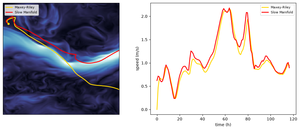

The §3.1 ensemble injected the unresolved scales as a Smagorinsky diffusion on position, with a diffusivity $K$ modelled from the local strain and amplitude $\sigma=\sqrt{2K}$ . The Maxey–Riley model lets us be more physical. A real float is dragged through unresolved turbulence, so the seawater velocity felt in the drag is $\mathbf v + \mathbf v'$ , with $\mathbf v'$ a sub-grid fluctuation; modelling $\mathbf v'$ as white-in-time turns the drag into a stochastic forcing on the velocity. Here $K$ is the ocean eddy diffusivity with $K=\sigma_v^2\,\tau$ , and the drag makes the slip an Ornstein–Uhlenbeck process whose stationary variance is $\sigma_v^2=\sigma^2\tau/2$ ; hence

\sigma=\frac{\sqrt{2K}}{\tau}

(5)

-- the same $\sqrt{2K}$ as in §3.1, now divided by the response time $\tau$ because the noise drives the velocity rather than the position directly.

Lateral stirring is anisotropic — stronger along the flow than across it (shear dispersion), so $K_\parallel>K_\perp$ . With $\hat{\mathbf e}_\parallel$ along the local seawater velocity, the diffusion maps a 2-D Wiener increment into the velocity leaf,

\Sigma\,\mathrm d\mathbf W = \frac{\sqrt{2K_\parallel}}{\tau}\,\mathrm dW_\parallel\,\hat{\mathbf e}_\parallel + \frac{\sqrt{2K_\perp}}{\tau}\,\mathrm dW_\perp\,\hat{\mathbf e}_\perp ,

(6)

a state-dependent, non-diagonal $2\times2$ operator. We express it as a lineax.FunctionLinearOperator returning a State tangent (noise on $\mathbf v_p$ only) and declare the 2-D Brownian space with brownian_structure.

import lineax as lx
from pastax import EulerHeun

NOISE_DIM = jax.ShapeDtypeStruct((2,), jnp.float64)   # 2-D Wiener (along/cross-stream)
C_PAR = 0.5     # along-flow Smagorinsky coefficient
C_PERP = 0.05   # cross-flow Smagorinsky coefficient


def maxey_riley_sde(t, y, args):
    forcing_ocean, forcing_wind, R, alpha, tau, c_par, c_perp = args
    drift = maxey_riley_drift(t, y, (forcing_ocean, forcing_wind, R, alpha, tau))

    w, _, _ = water_fields(forcing_ocean, t, y.x)
    speed = safe_sqrt(w[0] ** 2 + w[1] ** 2)
    inv = 1.0 / (speed + 1e-9)
    e_par = w * inv                              # along-flow unit vector
    e_perp = jnp.array([-w[1], w[0]]) * inv      # cross-flow unit vector

    # Smagorinsky strain |S| from a 3x3 patch of the smoothed current (cf. §3.1),
    # split anisotropically by a vector-valued C_S = (c_par, c_perp).
    patches = forcing_ocean.neighborhood(t, y.x[0], y.x[1], t_window=0, lat_window=1, lon_window=1)
    u_patch = patches["u_o"][0]
    v_patch = patches["v_o"][0]
    du_dx = (u_patch[1, 2] - u_patch[1, 0]) / (2 * DX_M_S)
    du_dy = (u_patch[2, 1] - u_patch[0, 1]) / (2 * DY_M_S)
    dv_dx = (v_patch[1, 2] - v_patch[1, 0]) / (2 * DX_M_S)
    dv_dy = (v_patch[2, 1] - v_patch[0, 1]) / (2 * DY_M_S)
    strain = safe_sqrt(2 * du_dx ** 2 + 2 * dv_dy ** 2 + (du_dy + dv_dx) ** 2)
    k_par = c_par * DX_M_S ** 2 * strain         # along-flow eddy diffusivity (m^2/s)
    k_perp = c_perp * DX_M_S ** 2 * strain       # cross-flow eddy diffusivity (m^2/s)

    # velocity-noise amplitude: sigma = sqrt(2K)/tau has units m*s^-3/2, so
    # sigma*dW (dW ~ sqrt(dt)) is a velocity increment (m/s) -> diffusivity K.
    sig_par = safe_sqrt(2 * k_par) / tau
    sig_perp = safe_sqrt(2 * k_perp) / tau
    Sigma = jnp.stack([sig_par * e_par, sig_perp * e_perp], axis=1)   # (2, 2)

    diffusion = lx.FunctionLinearOperator(
        lambda dW: State(x=jnp.zeros(2), v=Sigma @ dW), NOISE_DIM)
    return drift, diffusion


mr_ens = solve(maxey_riley_sde, state0, t0_sim,
               n_save_sim, INT_DT, int_dt_sim, solver=EulerHeun(),
               args=(forcing_ocean_smooth, forcing_wind, R_BUOY, ALPHA, TAU, C_PAR, C_PERP),
               key=jr.key(0), n_samples=100, brownian_structure=NOISE_DIM)
print("Maxey-Riley ensemble:", mr_ens.x.shape)       # (100, n_save + 1, 2)

Maxey-Riley ensemble: (100, 118, 2)

Animation — the stochastic Maxey–Riley ensemble (thin red) spreads anisotropically along the flow under the eddy-diffusivity noise, around the “true” inertial path (gold), over the evolving ocean speed and wind.

# Animation — stochastic Maxey-Riley ensemble over the time-evolving forcing.
ensemble = mr_ens.x

fig, ax = plt.subplots(figsize=(7, 5), subplot_kw={"projection": PC})
plt.close(fig)

o_speed = ocean_speed_smooth.isel(t=0)
time = o_speed.t.values
im = ax.pcolormesh(LON_S, LAT_S, o_speed, cmap=cmocean.cm.ice,
                   vmin=0, vmax=ocean_vmax, shading="auto", transform=PC)
fig.colorbar(im, ax=ax, label=r"$\| \widetilde{\mathbf{u}}_o \|$  (m s$^{-1}$)", extend="max")
q_w = ax.quiver(w_ds.lon0, w_ds.lat0,
                w_ds.u10.sel(time=time, method="nearest"), 
                w_ds.v10.sel(time=time, method="nearest"),
                scale=320, color="white", alpha=0.7, width=0.004, pivot="mid", transform=PC)

ens_lines = [ax.plot([], [], color="red", alpha=0.18, lw=0.6, transform=PC)[0]
             for _ in range(ensemble.shape[0])]
mr_line, = ax.plot([], [], color="gold", lw=2.0, label="Truth", transform=PC)
ax.plot([], [], color="red", lw=0.6, label="Stochastic", transform=PC)
ax.scatter([y0[1]], [y0[0]], color="gold", s=20, zorder=4, transform=PC)
ax.set_extent(EXTENT, crs=PC)
ax.legend(loc="upper right", fontsize=8)
title = ax.set_title(np.datetime_as_string(time, unit="s"))

def draw(k):
    global q_w
    field_k = k + 1
    o_speed = ocean_speed_smooth.isel(t=field_k)
    time = o_speed.t.values
    im.set_array(np.ravel(o_speed))
    q_w.remove()
    q_w = ax.quiver(w_ds.lon0, w_ds.lat0,
                    w_ds.u10.sel(time=time, method="nearest"), 
                    w_ds.v10.sel(time=time, method="nearest"),
                    scale=320, color="white", alpha=0.7, width=0.004, pivot="mid", transform=PC)
    for i, ln in enumerate(ens_lines):
        ln.set_data(ensemble[i, : k + 1, 1], ensemble[i, : k + 1, 0])
    mr_line.set_data(mr[: k + 1, 1], mr[: k + 1, 0])
    title.set_text(np.datetime_as_string(time, unit="s"))
    return [im, q_w, mr_line, title, *ens_lines]

HTML(animation.FuncAnimation(fig, draw, frames=ensemble.shape[1],
                             interval=80, blit=False).to_jshtml())

This capstone packs the whole framework into one physically-grounded model: a PyTree state $(\mathbf x,\mathbf v_p)$ for the second-order Maxey–Riley dynamics (fluid acceleration, Coriolis, lift and drag to a wind/water-weighted carrier); an operator-valued diffusion (lineax.FunctionLinearOperator) for anisotropic, flow-aligned turbulence that a diagonal g cannot represent; and a browian_structure decoupling the 2-D Wiener space from the 4-D state. Because the term is built from differentiable interp calls, the whole simulator is end-to-end differentiable — the parameters $(R,\alpha,\tau,C_\parallel,C_\perp)$ could be learned with the scoring rules of §3.2.

Where to next¶

See the API reference for the full surface of solve, Dataset, and the interpolation, metric, and score helpers.
The solve integrator supports both reverse-mode (jax.grad, used by BFGS above) and forward-mode (jax.jvp, used by Levenberg-Marquardt above) auto-differentiation. Reverse mode is the low-memory default (adjoint="checkpointed"); forward mode requires solve(..., adjoint="forward"), as in the §2.2 fit.

References¶

Aurélie, A. (2026). Champs de surface eNATL60. IFREMER. 10.12770/DD5D496A-8B55-4EAC-B989-F50B44BFC4AB
Pic, R., Dombry, C., Naveau, P., & Taillardat, M. (2025). Proper scoring rules for multivariate probabilistic forecasts based on aggregation and transformation. Advances in Statistical Climatology, Meteorology and Oceanography, 11(1), 23–58. 10.5194/ascmo-11-23-2025
Beron-Vera, F. J., Olascoaga, M. J., & Miron, P. (2019). Building a Maxey–Riley framework for surface ocean inertial particle dynamics. Physics of Fluids, 31(9). 10.1063/1.5110731